

According to the documentation, Pipe Query Syntax (hereinafter referred to as Pipe) is an extension of the SQL query language that is simpler and more concise than standard SQL syntax. Pipe supports the same operations as standard SQL syntax while enhancing certain aspects of functionality and usability. Before introducing Pipe, Google conducted research and provided a detailed explanation of it here. The following screenshot is taken from this research. It clearly illustrates the complex execution logic of a standard SQL query and how the same query appears in a more linear and logical form using Pipe.
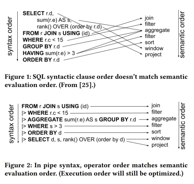
If you're anything like me, the previous information probably didn’t impress you much...
I consider myself quite a skeptical person who dislikes change. So the first thing that came to my mind when I saw the initial mentions of Pipe was: "Why reinvent the wheel? SQL is already the simplest programming language."
Additionally, I’m someone who likes to have a well-founded opinion. So, almost immediately after Pipe became publicly available, I decided to dive into it—just to prove to myself that Google had come up with something useless. My skepticism lasted about an hour. Unexpectedly, I realized that this syntax struck a chord with me.
But as always, let’s go step by step:
Structure and Purpose of the Article
I won’t go over the documentation. Instead, I’ll share examples of queries of varying complexity based on raw GA4 data, written in two formats—standard SQL and Pipe. Using these examples, we’ll analyze the differences so that you can decide for yourself which is better: the new syntax or the eternal classic. Though perhaps eternal should be in quotation marks...
Query 1 – Top 10 User Sources
Let’s start with something simple—identifying the top 10 sources that bring the most users to your website.
| SQL | Pipe |
|---|---|
|
|
I intentionally added a "human-readable translation" in the comments for each line of the query. Of course, the syntax is different, but visually, the "profit" isn't immediately obvious.
You might think: "I already know SQL well, so why should I spend time learning Pipe?" I had the same thought.
But try reading only the comments and ask yourself: "Which one is easier to follow?"
Overview of Key Operators
You may have noticed — or maybe not — that the previous Pipe query does not include the SELECT operator. In SQL, there are two mandatory operators: SELECT and FROM. In Pipe, only one is required — FROM. Essentially, SELECT * FROM table in Pipe is simply written as FROM table.
In this context, SELECT has lost its mandatory status and is now on the same level as other operators.
Here are some of the most commonly used operators in Pipe:
- |>AGGREGATE – Handles aggregation functions, which were previously performed in SELECT. It is used together with GROUP BY to define the parameters for aggregation.
- |>SELECT – Used to list the columns to be retrieved from a table. It can also rename existing columns and create new ones using simple non-aggregated expressions, e.g.:
x * y AS z
However, I don't recommend adding new columns in this operator since there is a dedicated one for that. The only additional use case for SELECT, apart from its primary function, is renaming a few columns—though RENAME exists for that purpose as well. If extensive renaming is needed, it's better to use the appropriate operator. - |>EXTEND – Used to add new columns based on existing ones. Yes, you could add them in SELECT, but the major advantage of Pipe lies in its readability. Using operators according to their logical purpose allows you to quickly understand the data processing flow—where columns are merely selected and where new ones are created. If everything were done "the SQL way" in SELECT, it would quickly make the query harder to read.
- |>SET – Unlike the previous function, it does not add new columns but modifies existing ones. It works similarly to:
SELECT * REPLACE (column * 2 AS column)
However, the syntax is different and more logical: column_name = expression:|>SET column = column * 2
- |>WHERE – Combines the functionality of WHERE, HAVING, and QUALIFY. Now, you don’t need to decide which of these three operators to use for filtering—if you need to filter something, |>WHERE does the job.
- |>JOIN – Works exactly the same as in standard SQL—it joins tables.
- |>UNION – Functions just like in traditional SQL, appending data from the second table to the first. By adding BY NAME, for example:
UNION ALL BY NAME. The union will be performed based on column names, regardless of their order in the tables. This significantly reduces the likelihood of errors during the merging process, effectively bringing it down to zero.
By the way, the UNION ALL BY NAME option was also added to standard SQL around the same time Pipe became publicly available. You can find more details here.
But these are not all the operators. You can find the full list here. As you can see, there aren’t too many of them, and they all have logical names. This means that when reading a Pipe query, you can already anticipate what kind of processing will occur in the next block—of course, as long as you use the commands as intended. :)
You may have noticed that operators begin with the |> symbol. This marks the start of the next processing step. These can be added indefinitely, eliminating the need to create numerous subqueries and come up with names like "raw", "prep", "final", "super_final", "last_final", "the_very_last_final_I_promise", or "final2".
The |> symbol is not added before FROM, as it marks the beginning of a query rather than a step. It is also not used before GROUP BY, as that is part of the AGGREGATE operator.
Query 2 – Most Popular Pages on the Website
That’s it for the theory. If you were already familiar with SQL, it should take you roughly 1–2 hours to grasp the principles of Pipe and practice using it.
Now, let's look at the following query, which will show us the 10 most visited pages.
| SQL | Pipe |
|---|---|
|> |>AGGREGATE
|> |> |> |
In this example, it’s clear that standard SQL requires extra "work." We need to jump to the WHERE clause to understand why COUNT(*) is labeled as pageviews. Additionally, to calculate the rate, we have to repeat the formulas for counting page views and users.
With Pipe, you follow the logical processing sequence step by step, and in later stages, you can directly use column names that were already defined earlier.
Query 3 – Open E-commerce Funnel with Breakdown by User Browsers
The following query will help you determine whether there are potential technical issues in the funnel for a specific browser.
| SQL | Pipe |
|---|---|
|
|>
|
And when queries become a bit longer, another small profit becomes evident—queries in Pipe are generally shorter. While not always the case, in the vast majority of situations, they tend to be more concise. Based on my tests, Pipe queries are about 15–20% shorter, and in some cases—especially when processing data from a single table without joins—they can be up to 40% shorter.
For large queries, this is a significant advantage, as you maintain a clear processing logic and spend less time jumping between different subqueries.
Query 4 – GA4 Traffic Acquisition Report
Finally, let's look at an example query that retrieves data from what is likely the most popular report in GA4—Traffic Acquisition.
| SQL | Pipe |
|---|---|
|
( ( (
|>
|> |
As I mentioned earlier, Pipe queries are not always shorter, but they maintain a sequential and linear structure that is significantly easier to comprehend compared to standard SQL.
You may have noticed that in this example, for simplicity, I used the primary_channel_group field from the session_traffic_source_last_click.cross_channel_campaign object. This field is relatively new and is supposed to reflect traffic channel values from the GA4 interface, where sources are determined based on the last known source. However, I have many concerns about the GA4 interface—it is, to put it mildly, not perfect.
Previously, I conducted research on other fields within this object—specifically session_traffic_source_last_click.manual_campaign, which appeared slightly earlier—and compared them with the GA4 interface. The results for some projects were quite surprising. You can find the link to that research here.
A different approach is to use raw, unprocessed Google data instead of relying on predefined values. The true foundation for determining traffic sources lies in page_location and page_referrer. While processing logic based on these fields is undoubtedly more complex, it can help fix interface bugs and customize data to meet specific business needs.
At one point, Max and I hosted a webinar, where we thoroughly analyzed how GA4 determines sources in the interface and shared a script based on page_location and page_referrer. You can purchase access to the recording and script here.
And if everything written above sounds like "very interesting, but totally unclear" to you, then your best bet is to join the BigQuery for Marketing course. There, the sensei instructor, with his expert teaching skills, explains complex topics related to working with raw data in BigQuery in an easy-to-understand manner.
Final Thoughts
I hope that through these examples, I was able to introduce you to the principles of Pipe and highlight the differences between it and standard SQL.
I'm certainly not trying to persuade you to "join the dark side." I firmly believe that learning the classic SQL syntax should come first, as it is the most widely used. With some variations, SQL is applied everywhere data processing is needed. However, these "variations" do not affect the query execution plan, which remains consistent across different dialects.
And here comes the "but." Pipe has a significant advantage—it is simpler and more logical. This makes it easier for more specialists to start working with raw data, as learning and understanding Pipe takes less time.
For those already working with data, the simplicity and sequential nature of this syntax improves comprehension of processing stages, which in turn reduces the likelihood of errors when writing complex query logic.
To summarize my impression of Pipe, I can confidently say that Google didn’t come up with nonsense! :)
Loading comments…